In this page, we show our numerical experimental results based on bivariate spline functions for image enhancement. See our paper : Q. Hong and M. J. Lai, Bivariate Spline Approach for Image Enhancement" on www.math.uga.edu/~mjlai/indexPublications.html for technical details.

Bivarite splines are piecewise polynomial functions over triangulated domain with smoothness r and degree d with d>r. See monograph on multivariate splines by Lai and Schumaker for theory and approximation of bivariate, triangulation, and spherical splines. See paper on numerical algorithms for how to use bivariate and trivariate splines for data fitting and numerical solution of PDE's. See paper for numerical algorithms for data fitting using spherical splines.

Numerical results are organized in following categories:`

image triangulation;

Image inpainting and stain removing ;

image reconstruction from 5% and 1% random samples

image resizing ;

image denoising ;

image wrinkle reducing;

image edge detecting;

For image/movie denoising based on framelets and sparse representation, see here.

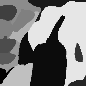
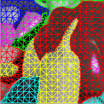
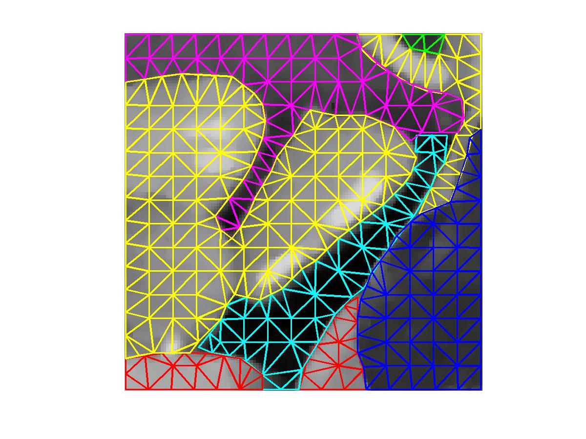
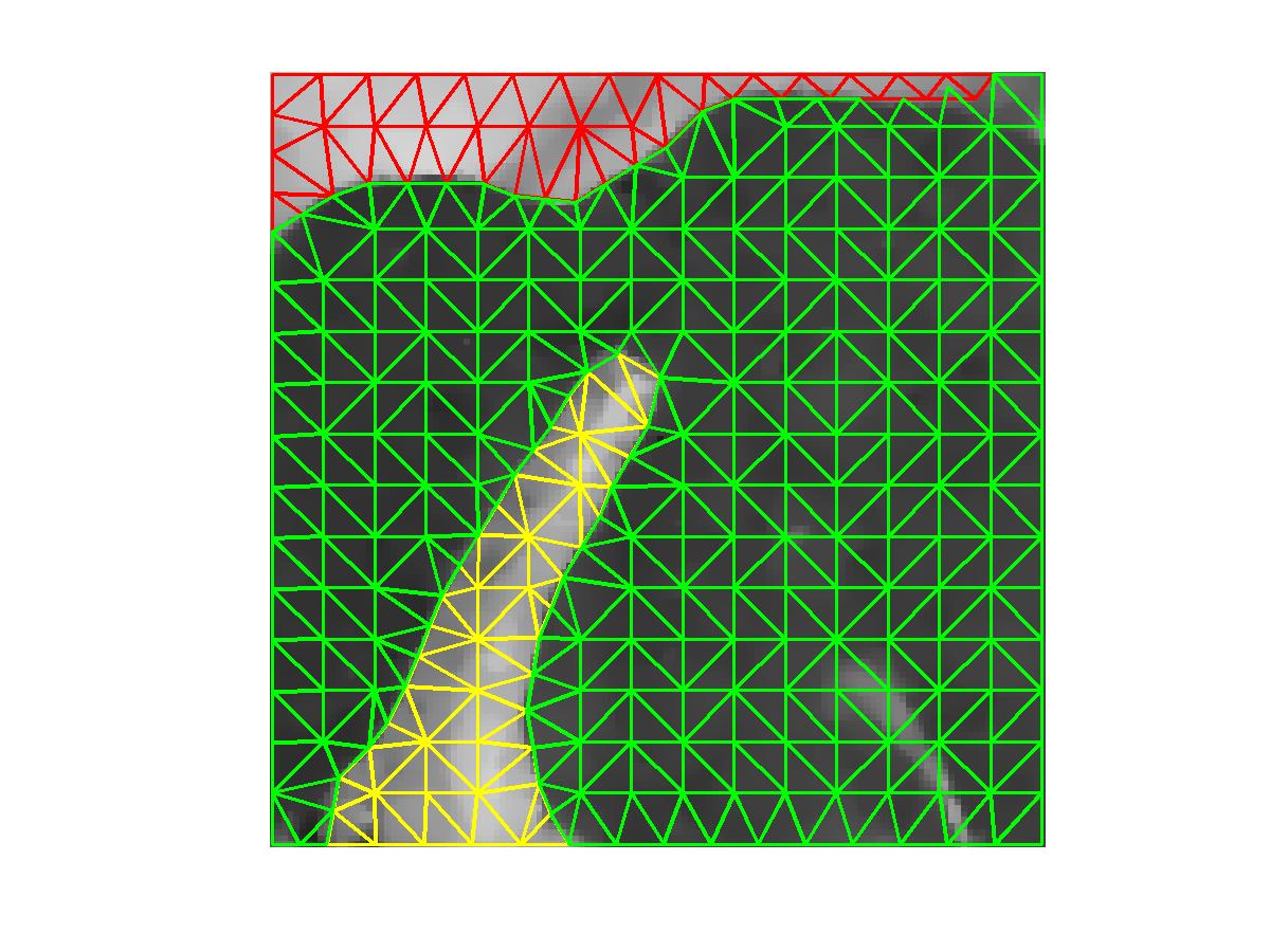
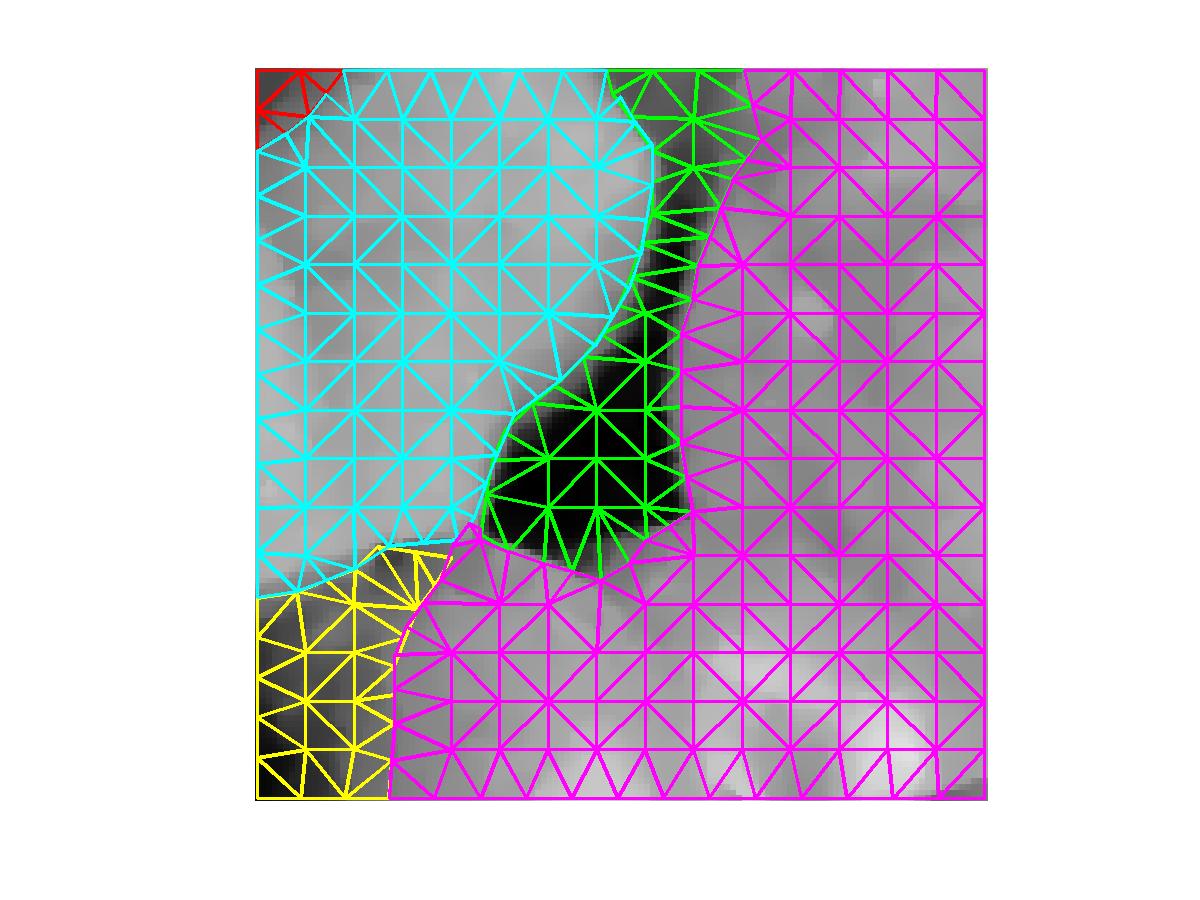
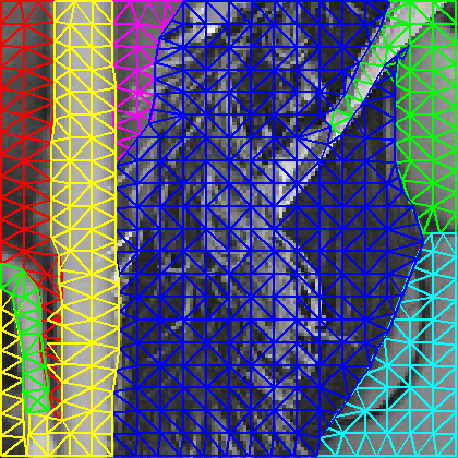
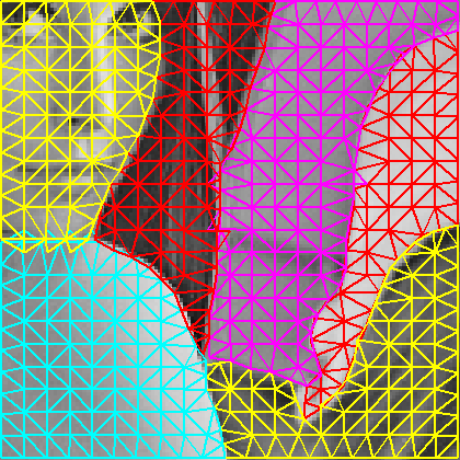
Example 1. Image Triangulation. We first use the active contour algorithm ([T. Chan and L. Vese, Active Contour Without Edge, IEEE Transactions on Image Processing, 10(2001), 266-277]) iteratively to decompose an image into several regions and then triangulate each region automatically with adjustible parameter for the size of triangles.

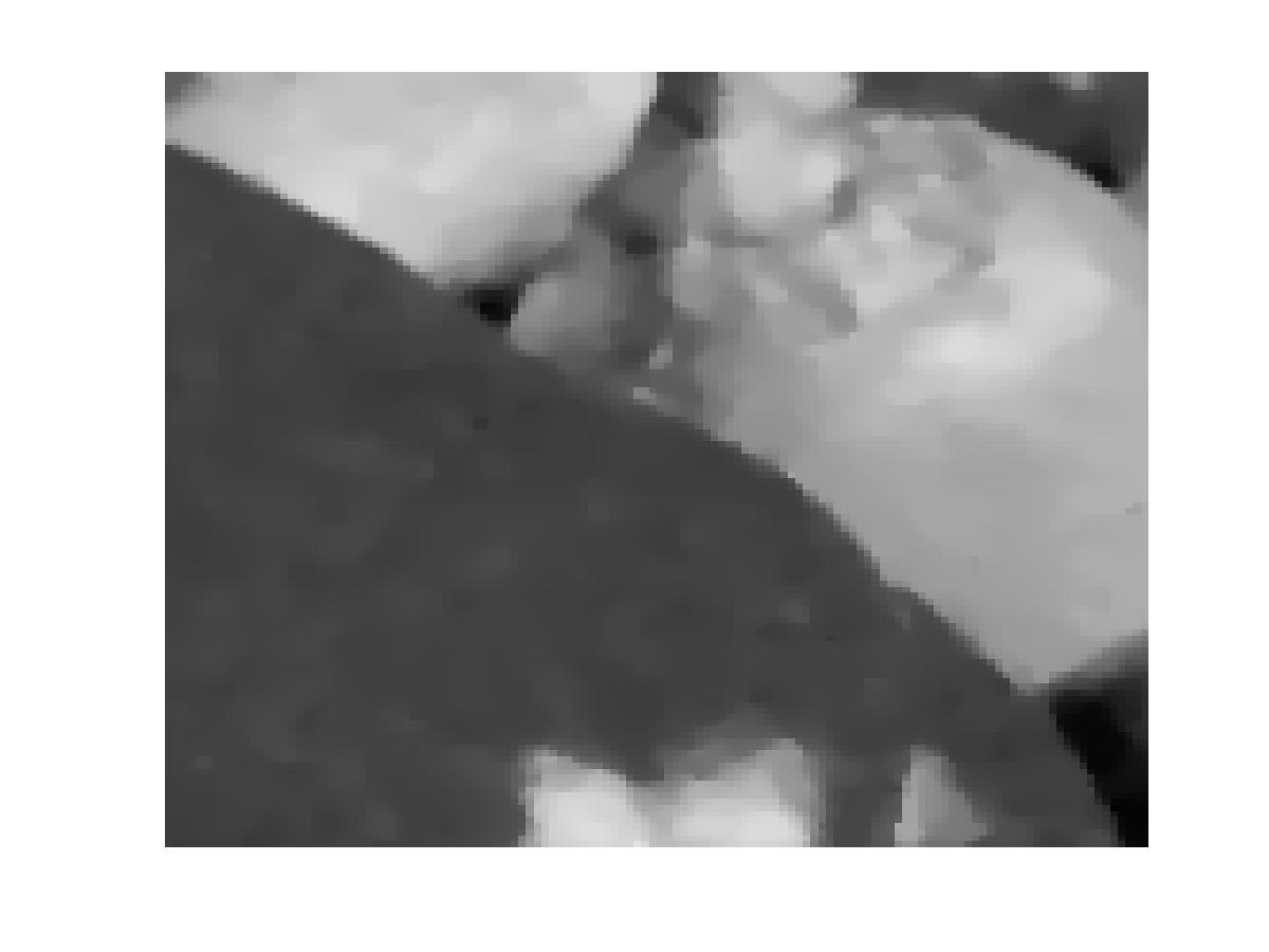
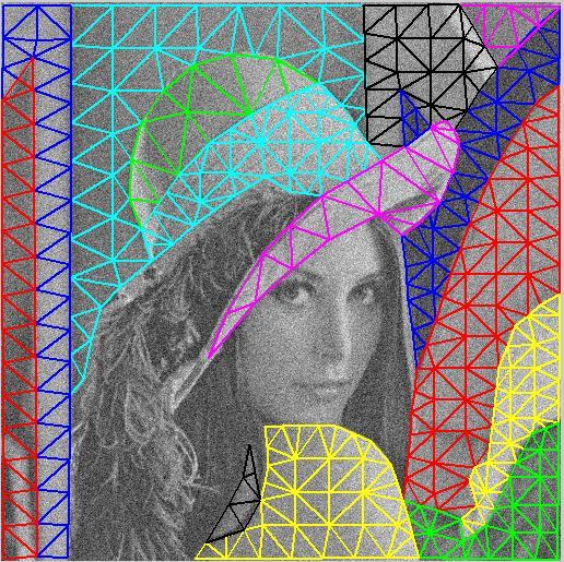
Here are more examples:

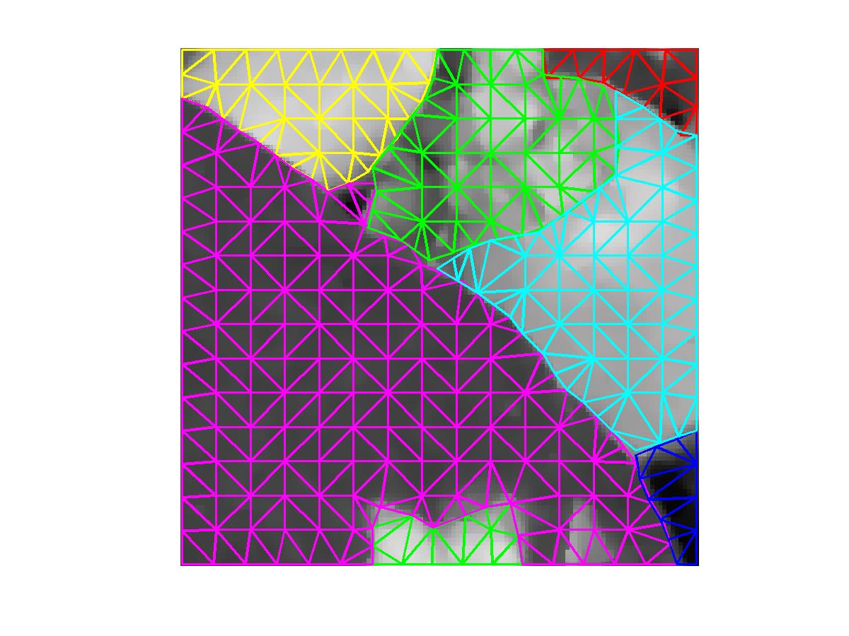
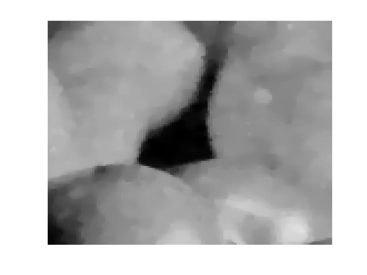
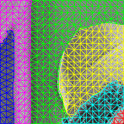
Here is another example:

More examples can be found in Q. Hong's dissertation.

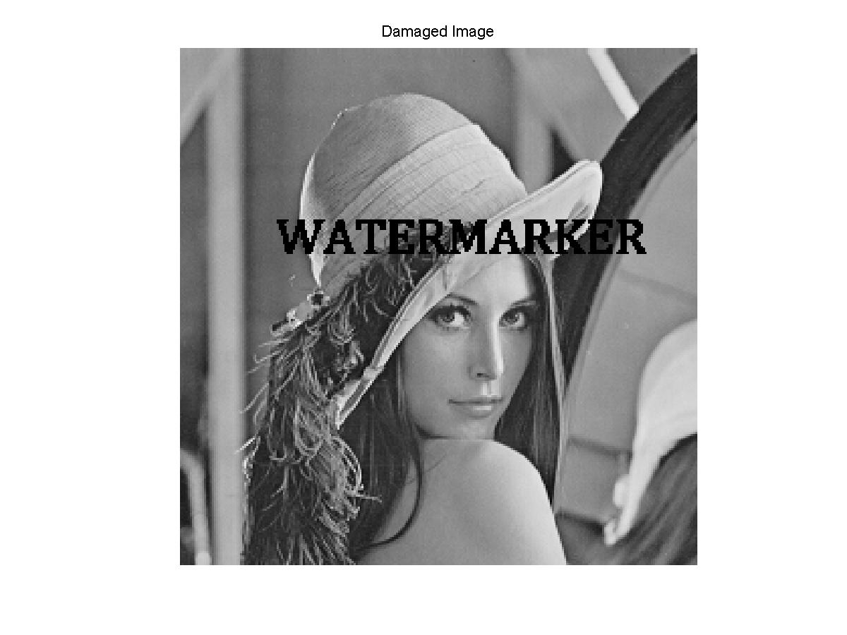
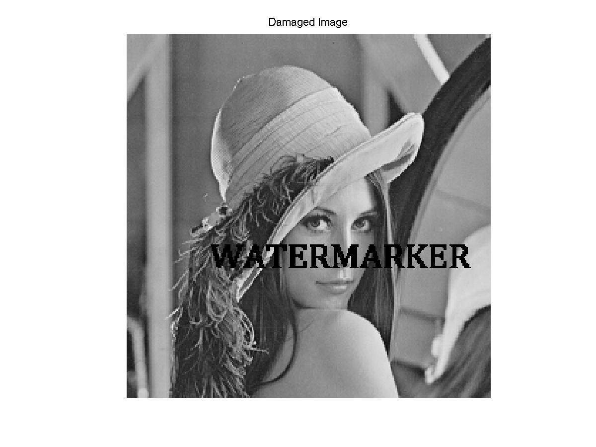
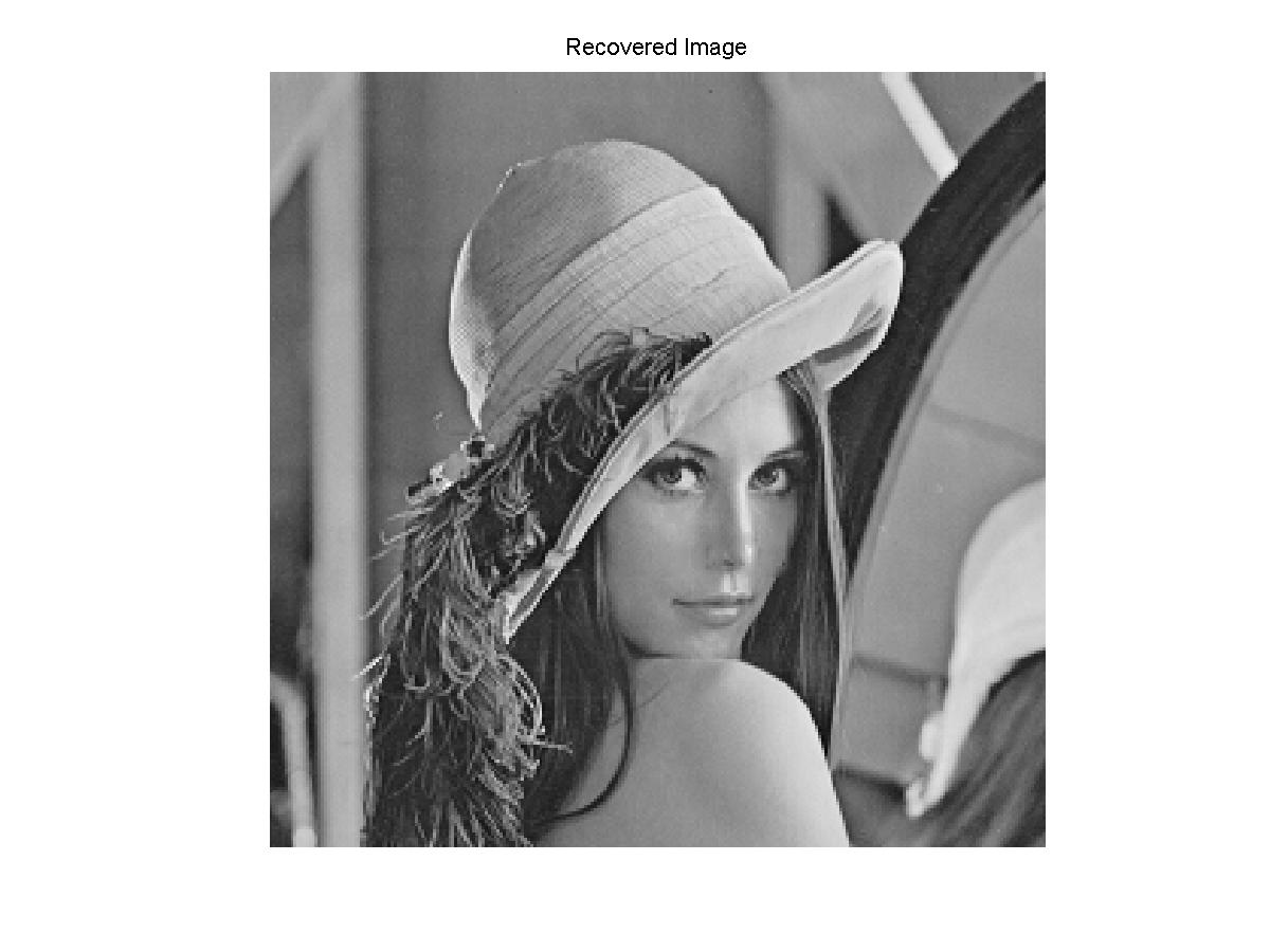
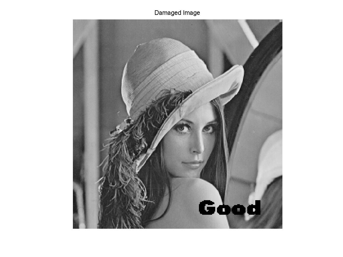
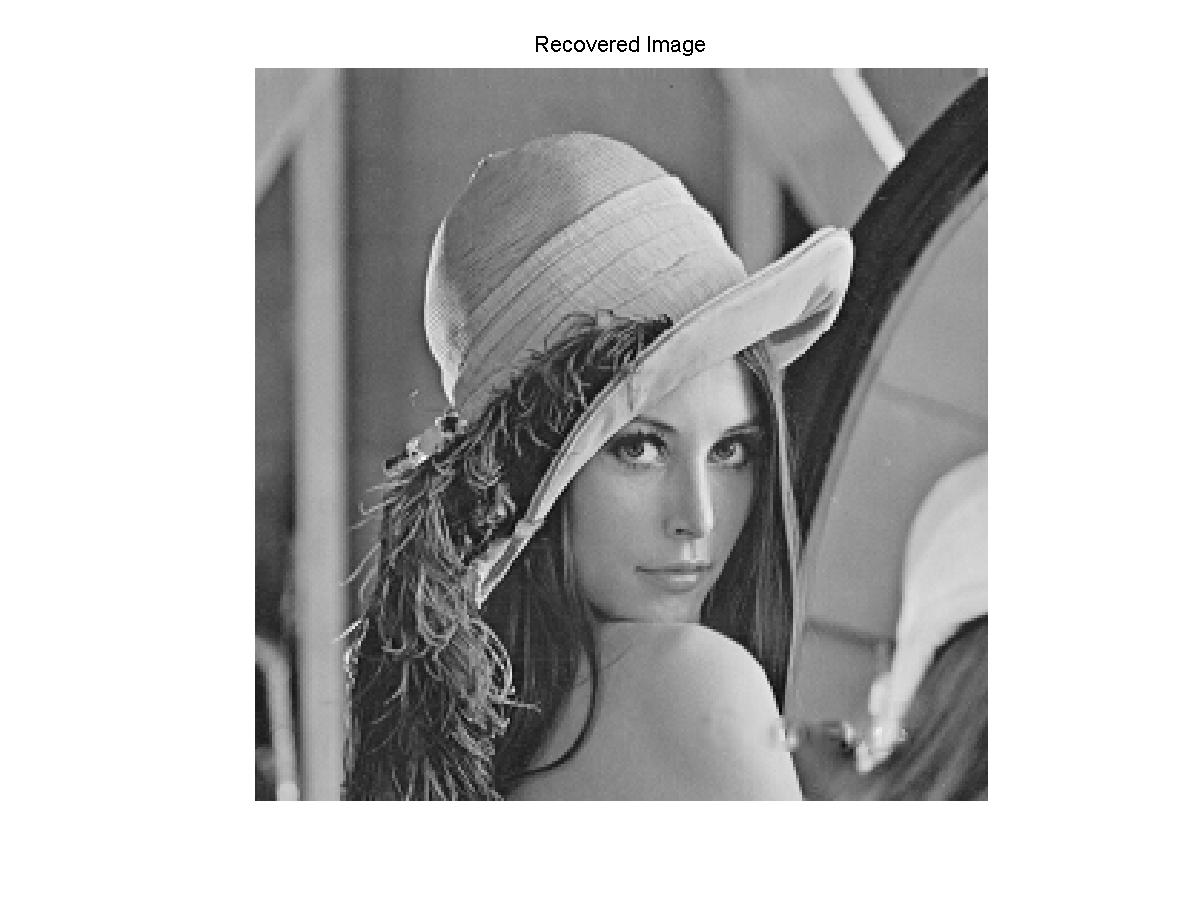
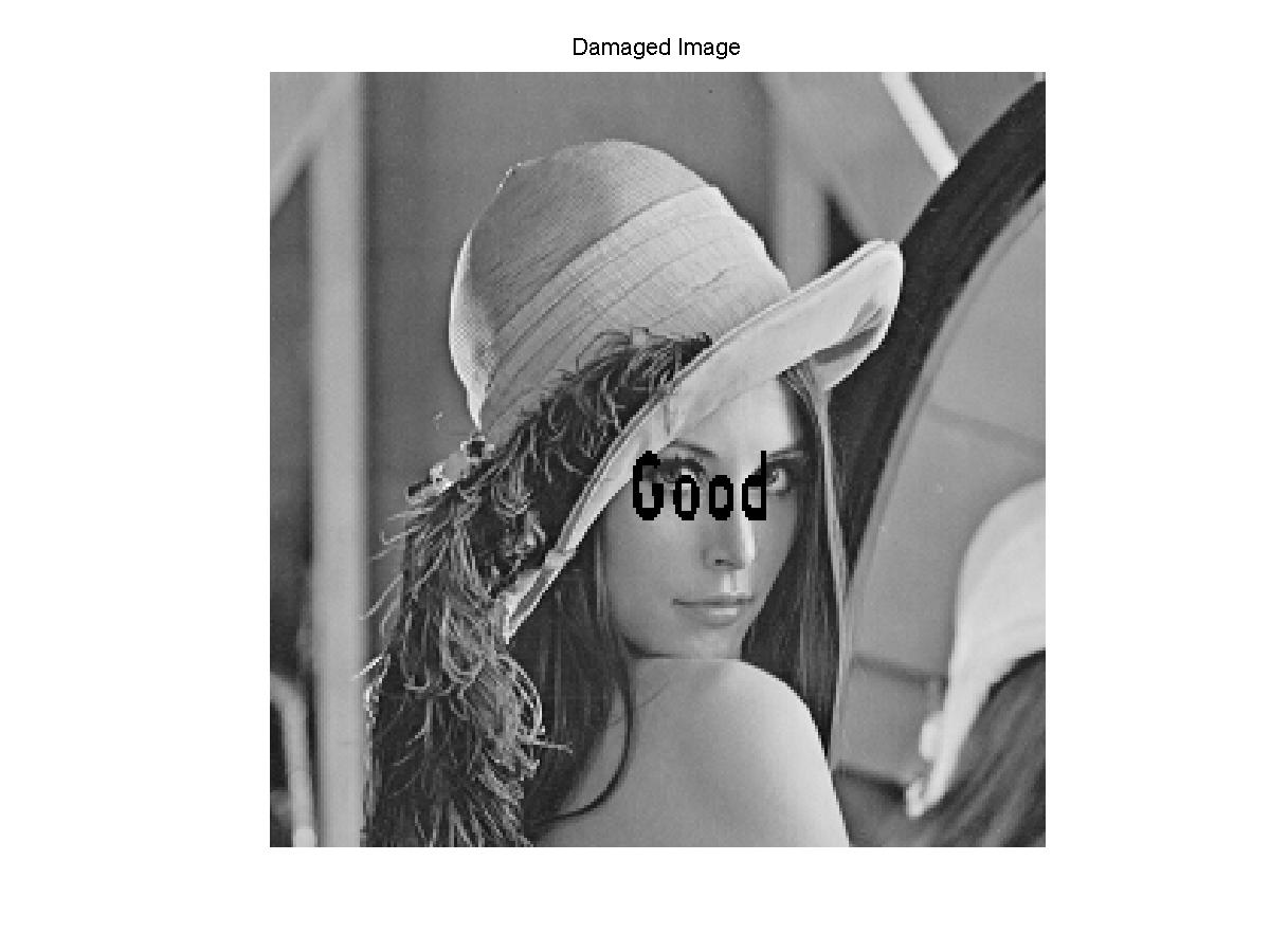
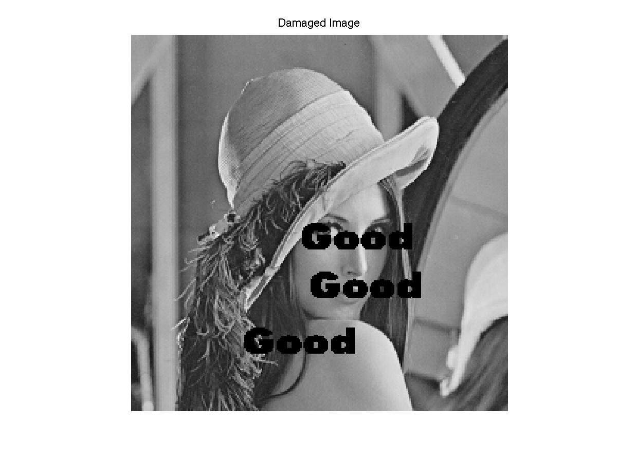
Example 2. Image Impainting and Stain Removing: We first damage the images in various places and then recover the images using the minimal surface area fitting splines.

Example 3. Image Reconstruction based on 5% Random Samples. We randomly sample 5% of the image values based on uniform distribution from standard images, e.g. lena.pgm and pepppers.pgm. We use bivariate splines to reconstruct an image function from the scattered data values based on the minimal surface area approach. With \lambda=0.1, \lambda=1, and \lambda=40, let us see what we are able to recovery from the 5% of original images.

Next we show what we can recover from a set of 1% random samples.

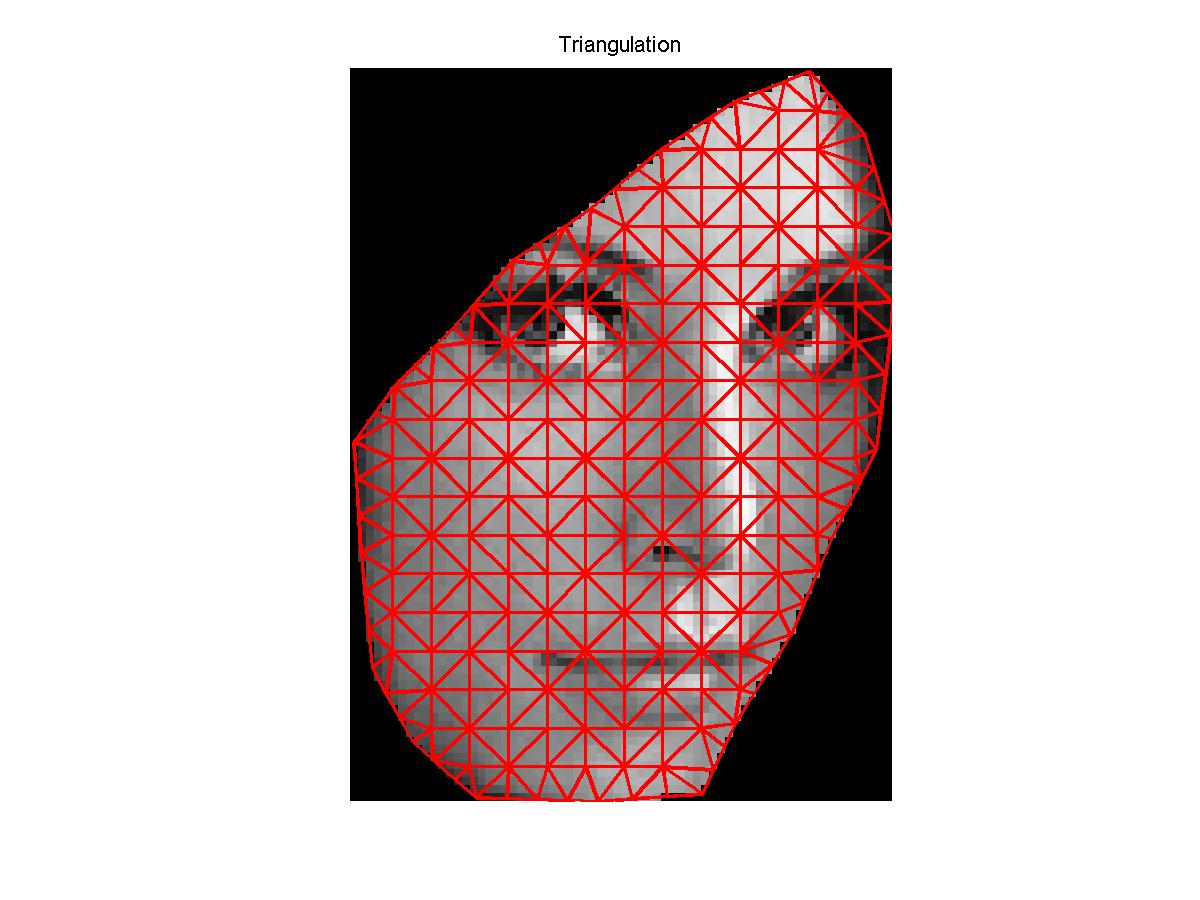
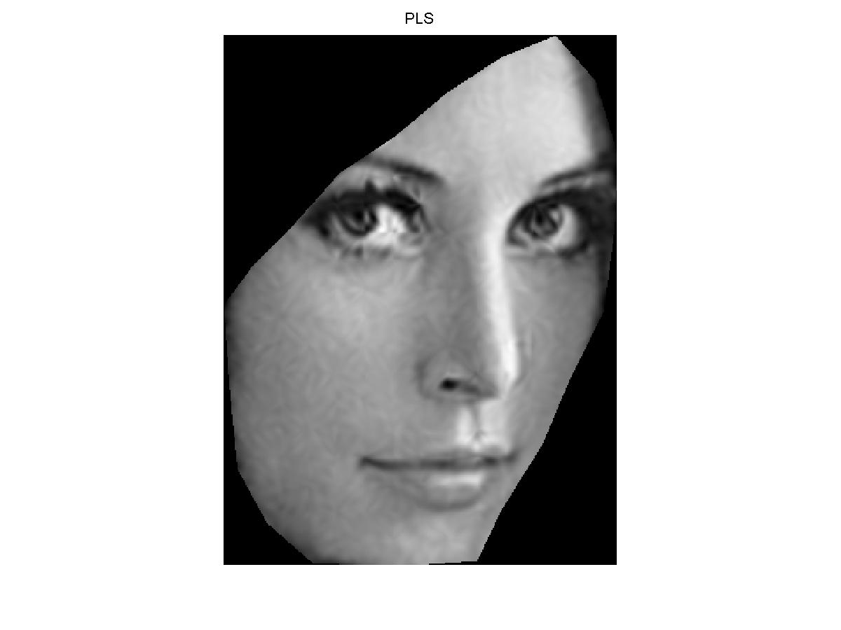
Example 4. Image Resizing: We choose the face of a standard image Lena and find a triangulation. Then we apply two fitting schemes: one is the standard penalized least squares (PLS) fit and one is the minimal surface area (MSA) fit. The figure in the middle is based on MSA which is smoother than the one next which is based on PLS.

Here are two more examples to show that our method is better than the standard bilinear and bicubic splines.

Original	Minimal Surface Area Fitting Spline	Bicubic Spline	Bilinear Spline

More examples can be found in Q. Hong's dissertation.

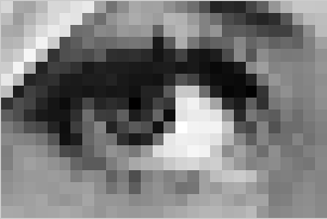
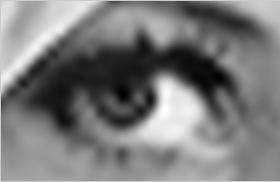
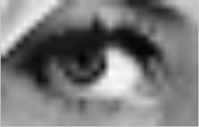
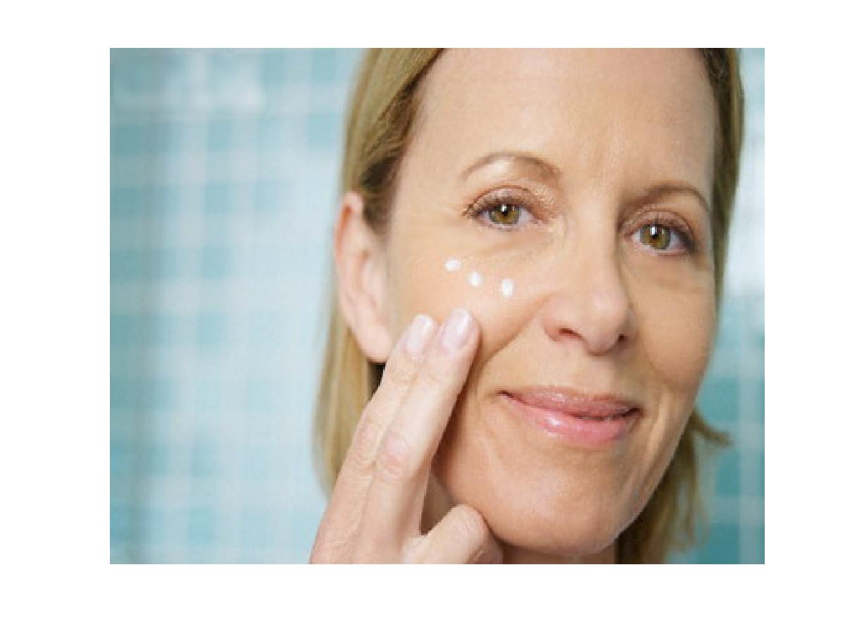
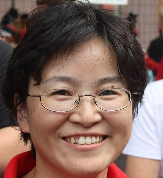
Example 5. Wrinkle Reducing: We use the minimal surface area fit based on bivariate splines to reduce the wrinkles around the cheeks and eye corners by first selecting a region to enhance, triangulating the region, applying minimal surface area spline method to obtain a fitting spline and then using the values of the fitting spline within the region to replace the pixel values. Enhanced image will have much less wrinkles.

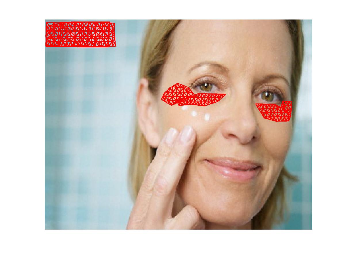
Original
MSA Splines

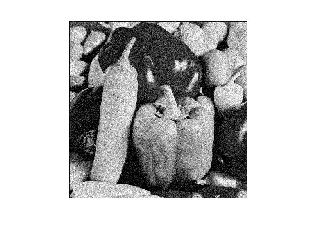
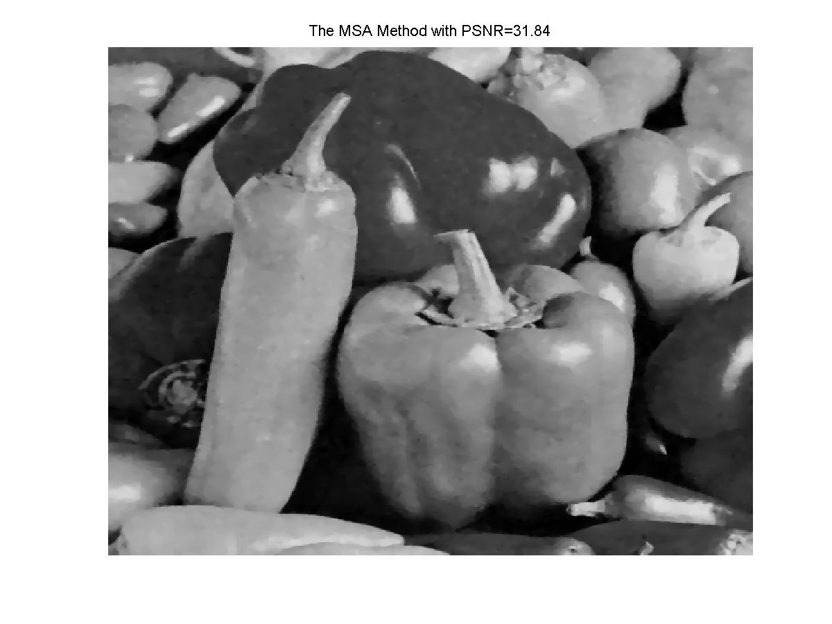
Example 6. Image Denoising: We add Gaussian noises 20 N(0,1) onto a standard image Peppers to generate a noised image. Then we apply our MSA fitting splines to remove noises from each triangulated region. The noised image and de-noised images are shown below. The PSNR is 31.84.

However, I am not pleased with this numerical result as much better results can be found in this link.